All posts by Erick Clasen

sellbuy-o-meter

The Golden Ratio Multiplier Trading Algorithm

This post covers a trading algorithm developed in Python code that uses Fibonacci numbers to set levels to trade off of. It is not a short term strategy, however it is a long-term strategy more of an investment strategy. It is based on a post by Philip Swift on https://www.lookintobitcoin.com/charts/golden-ratio-multiplier/

And he also has an original article on it on medium.

https://medium.com/@positivecrypto/the-golden-ratio-multiplier-c2567401e12a?sk=e38c4eff4357a1131bed57a3f4b3eeae

I have code for this here:

cbpro-cli-tools

Theory

The golden ratio multiplier is a great indicator, visually easy to confirm and makes a lot of sense on how it works. Best of all no fussy back-testing with parameter tweaks, you just need your eyes. I like how Josh Olszewicz  added the centerline, that is a nice addition. His video was a pleasant and positive surprise that I used to review the working of the golden ratio multiplier. I started using this indicator in early 2020.

On top of the basics that are covered by Phillip Swift , I have made some additions to the it that will work well in algorithmic form to allow it to run with constraints as code. Constraints are needed to allow it to pick the correct points to enter and exit along the curve. The method of (Dollar Cost Averaging) DCAing in and out is to use 20SMA BBands (Bollenger Bands) as a point to trigger DCA, using this as a filter to trigger on price exceeding lower/upper BBand. This tweak is based on the fact that I wrote code around this and was looking for a good way for when it should reasonably DCA, versus just triggering on a crossing the Fib # * YearlySMA (SMA, Simple Moving Average), or DCAing daily when under/above this line. As far as amounts to DCA, generally with accumulate/distribute investing, I tend to compound the trades in a way that accumulates heavier as distance increases below the YearlySMA line and distributes heavier as it goes further above the target Fib # * YearlySMA. The trading scaler used is a logistic curve , with n being the ratio of the current price to the yearly avg for buys (For sales ‘n’ is inverted by n being subtracted from the target Fib level multiplier + 1, which positions the curve out to where it scales up until it reaches the next higher Fib # and back down. Using the logistic curve formula (1+k)/(k + n^e) as a trade multiplier, for example with k=0.2 and e=4, it DCA’s in around 2x at the 0.8 * yearlySMA point,, 4x at 0.5…never more than 6x as it approaches that as a limit as n –> 0. I am planning publishing this code and documentation around it and will cite your video in it when I do.

Golden Ratio Multiplier Tutorial

Also Josh Olszewicz has a video tutorial on YouTube about this particular indicator using it with TradingView code it is a worth taking me 10 minutes or so to review this as background material along with looking at https://www.lookintobitcoin.com/charts/golden-ratio-multiplier/ and the original medium article . I am going to try to stick to the essence of the code and not so much the background material which could be read in viewed in those locations.

Code

This code is light weight and can be run on a Raspberry Pi as well as a Linux PC. It requires Python 3 as this is needed for the API.

The code is designed to use the Coin Base Pro API, however there is a middle layer that interfaces with the API via cbpro_buy_sell.py  If someone wants to interface with another API this just needs to be modified to make the proper calls into another exchange as an API on the back end of it. Think of it as a thin interface layer that goes between the code and the API itself.

cbpro-cli-tools

Dependancy : One import

this would be the import cbpro code that constitutes the module for the CV pro interface API.

Other Internal Dependancies

There are a few dependencies in the code thankfully they are local dependencies. The intent was to make this code as freestanding as possible without having to import various library’s other than what is barely necessary to make it operate. The first is a file called coretamodule.py. It holds a lot of functions that are used in multiple algorithm some of which will be used in the code to implement the golden ratio multiplier which is known as the arc just Python. The other necessary dependency is a piece of code that calls for polls periodically the CB pro ticker to add prices and volumes to aC SV file. This is run from some thing like Cron on a regular basis hourly daily five minutes what have you it is run at the same rate as a fib-ad high is run calling this code 1st to fill in the CSV file which will be read in by fib active high. I will try to make this publicly available on a site where it could  be pulled down with that lease this up to the current days data. Current days data

Core concepts

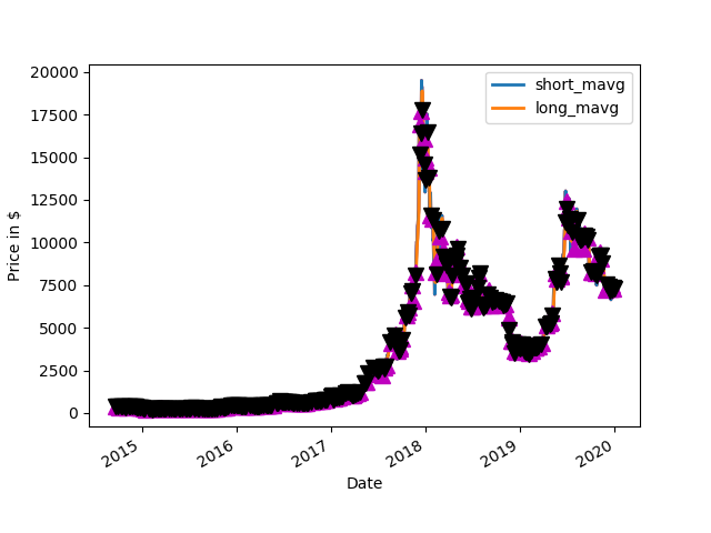
The idea of the code is that a 350 day moving average is calculated.This forms the basis of the ratio that is the golden ratio between the average and the price itself. When the price is below a threshold which is coded in to a dictionary of two pools as one. When below this level it will accumulate in the particular currency pair. There is another number in this threshold when it is above this ratio of price to 350 day moving average price. this forms the basis of the ratio that is the golden ratio between the average and the price itself. When the price is below a threshold which is coded in to a dictionary of tuples as one. When below this level it will accumulate in the particular currency pair. There is another number in this threshold when it is above this ratio of price to 350 day moving average price.above this range it will distribute the currency pair. Some fine tuning is made when it is above or below the threshold. The fine-tuning is based on Bollinger bands when it is touching the bottom bands in the Bollinger band 20 day bands and the minimum price for the 20 day period is also the same as this the price they buy is initiated.C onversely for the sale when the price is at the upper edge of the Bollinger band and the maximum price for the 20 day. Has been hit as a target a sale is initiated. This makes it dollar cost average in and out on a periodic basis. The idea is to have extra filtering to kind of find a peek in the valley of price movement without DCA (Dollar Cost Average) in too much or out too much.

defines.py

there is also a dependency file called defines.py this file has the portfolio amount in it. Now it is being dynamically allocated by using the cbpro_read_accts.py.  It will scale the amount of USD traded however BTC an ETH have to be adjusted within the main function to pick values that are comfortable and proper for the trading circumstances. This allows for configuration between all of the pairs.Also in the defines file you will have to enter the key passphrase and be 64 secret, this will allow the trades to occur through the API as this is passed on by the main code.


Also in the defines file you will have to enter the key passphrase and be 64 secret, this will allow the trades to occur through the API as this is passed on by the main code.


Outputs and Logs

The output from the code is interpret able humanly to understand what is going on as well. There are rose of prices after the initial currency pairs listed these prices represent the various thresholds at the end it states whether it is holding or not and also what the threshold and target are the threshold being the Bollinger bands edge and the target being the lowest to highest price for the 28th time.Additionally there are log files created when the code runs there are several that are verbose and specific to a underlying currency and there is one summary file. The verbose files contain the returned output from the API function call which is a dictionary of values return from CB pro. There will also appear within the non-verbose output as a message usually relates to some thing that needs to be corrected possibly a bug or some thing like insufficient funds. This is driven by the message key from the CB Pro API return dictionary.


The code makes every  attempt to avoid this because it uses limit orders and it also checks the balances in the supply. The underlying currency and the to be bought or sold currency itself.

Compounding Positions

There is also a logistic scaler in this code. The logistics scaler works by increasing the amount of currency bought when the price falls below the threshold of the golden ratio multiplier which is by default one. This allows increasing the amount purchased automatically but also reaches a limit as the ratio between the price and the 350 day moving average approaches zero. It will go to a limiting constant. The opposite is true for cells there is the threshold that is coded into the dictionary of tuples the logistic scaler takes in that value plus one informs a curve that goes from the upper threshold to all 1+ this value and increases the amount sold after this plus one position it will decrease once again to zero. The idea is that it scales out hard as the price rises but has a limiting factor if it rises above the threshold too far. The idea would be to manually address these thresholds to what is expected of the currency. So periodically maintenance might be required on the threshold or they might just be a set it and forget it for some people. This all depends on how you want to invest.


As the price rises but has a limiting factor if it rises above the threshold too far. The idea would be to manually address these thresholds to what is expected of the currency. So periodically maintenance might be required on the threshold or they might just be a set it and forget it for some people. This all depends on how you want to invest.The default or one and two in a two pole for every currency pair. It is possible to adjust days as needed. It is also possible to adjust the logistics scaler Constants which are KNEE is the exponential constant which controls the rate of rise of the curve and key controls the multiplier affect in the amount that would be traded in the limit.

Outer Loop

The code works by looping through a list actually a dictionary of underlying currencies US D/ETH/BTC as underlyings. Then there is a function call and the inner currencies are called in a loop these other currencies that are actually traded against the underlying currencies. This allows money currency pairs to be traded and others to be added in the future.

CSV Data Collection using API

The caveat here is that there has to be enough data in the CSV file to go back for the time. And if a currency one is to be added it has to be attitude there to harvest the ticker data. I suppose in theory it would be possible to fit all data into the file itself to add a prior prior currency that’s been running in the ticker for a while if someone is motivated not to do that. Having this code in a folder and having it called by Cron preferably using a script calling the script first then harvesting the price volume data then calling for code it will work seamlessly as a plug and play algorithm. Because it is using the golden ratio multiplier there is no need for back testing as this has been proven out to work by Philip Smith Swift in his presentation and write up online.

Obviously this code could be modified in anyway the 350 day. Could be changed to something else along with the 20 day Bollinger band. And the threshold as I said earlier our configurable.


11hp Briggs and Stratton

11hp Briggs and Stratton Carburetor Adjustment

Turn needle valve (high speed) clockwise until it closes. Do not force, stop when screw closes. Now open needle valve 1 1/8 turns counterclockwise. This will permit engine to start and final adjustment can be made after engine warms up.

– FINAL ADJUSTMENT Place governor speed control in “FAST” position (that means open throttle all the way). Turn needle valve in clockwise until engine slows(lean). Then turn it out counterclockwise past the smooth operating point(rich). Now turn the needle valve to the midpoint between lean and rich. Next adjust the idle mixture. Rotate the throttle counterclockwise and hold against stop.Adjust idle speed adjusting screw to obtain 1750 RPM. Holding throttle against the stop turn idle valve in (lean) and out (rich). Set at mid point between lean and rich. Re-check idle RPM. Release throttle. If engine will not accelerate properly, the carburetor should be re-adjusted, usually to a slightly richer mixture.

BTC Gains

BTC versus Stock Bull Run

Stock Bull Run
Stock Bull Run to Bust, 2009-2020

This post is an addition to the series on DMAC algorithm trading, which is simple algo trading example. I was wondering now that the S&P500 and etc, legacy market has dropped out of it’s long bull run, how would Bitcoin gains compare against the stock market?

First Post in Series to Learn More Background

Code to run this model on Github

BTC Buy and Hold -v- S&P 500 Buy and Hold

The plan: Comparing  Bitcoin (BTC) gains from January 1,2010 to December 31,2019 against the bottom for stocks on March 9, 2009 to Feb 19,2020, the 400% bull run for the S&P 500. But, for some reason the Yahoo data for Bitcoin is only going back to 2014-09-16. So we are basically getting a bit short changed here on BTC and giving the S&P a long head start for nearly 5 years. (I am sure at one point in the past, I think this used to work and go back all the way to 2010 but Yahoo must have cutoff the data since I first tried this code.)

So with 5 years head start for S&P

S&P500 4x gain across history shown in the above chart 03-09-2009 to 2-19-2020

BTC 16.96x gain from 9-16-2014 to 2-19-2020

Now for a true side by side comparison

S&P 500 on 9-16-2014 closed at 1998.98

S&P 500 on 2-19-2020 closed at 3386.15

S&P 500 gain 1.69x from 9-16-2014 to 2-19-2020

So Bitcoin beats the S&P using by and hold across the same time frame by 10x.

Buy and Hold -v- DMAC Algo Trading on BTC

OK, now what about BTC HODL (Buy and Hold) gains versus optimized DMAC algorithm trading from 9-16-2014 to 2-19-2020?

HODL Gains: 16.96393901373665

Algo gains for a 1 day short and 4 day long average. This is wicked tight and it will trade like mad, so in real life, the transaction fees and slippage would eat away at this number after 10 years.

Short AVG,Long AVG,Best Bank 1 4 2244962.564086914 which is 22.4x

which is 22.4x gains. But, with fees/slippage  and HODL at ~17x , HODL is really great. Beats the 4x or 1.69x depending on the time frame of the S&P 500!

It could do better

This is a simple algorithm, one of the simplest ones that can be thought of. Also, remember that the algorithm only tuned once across the entire time period. If the time  period was cut up into smaller periods and the algorithm learned the market as it changed over time instead of trying to get a best fit across 5 years it would have produced more gains. The example the initial post which has it trade from Jan 1 to Dec 31 of 2019 shows in making 900K alone in one year. So an algorithm that could in theory re-optimize periodically as the market conditions change would easily beat the results of this simple algorithm. The best thing that I can think of would be a machine learning algorithm that would use differential evolution to change the parameters as time goes on. It would learn on an ensemble of random sections of random lengths of data from the past and tune the algorithm’s parameters based on learning from the data ensembles. That is just one way that comes to mind.

But, at the end of the day this is just an example. It is not always possible to predict future results from past data. It is also well known and Covid-19, The Great Recession and Black Monday in 1987 serve as examples, there will be price shocks that can upend any model in practice. The statistics of price action do not fall neatly under a bell curve but have fat tails that lead to excursions far away from the mean on occasion. One only has to look to history for this lesson and one example is the firm Long-Term Capital Management (LTCM) led by a brilliant team of folks including Nobel prize winners Merton and Scholes, two out of the men that invented the Black-Scholes option pricing formula. Fischer Black, the other man was not alive at the time that the prize was awarded. Some credit for  the formula rests with Ed Thorp as well, at least a way in the backstory. Ed Thorp had basically the same kind of formula running on convertible bonds, not a far jump to options pricing. This is all outlined in the great book The Quants by Scott Patterson. Quants was one of the seeds that led me to pursue trading, specifically algorithmic trading a few years after I read it.

Lessons To Be Learned

So there were brilliant guys were at the heart of LTCM but, due to high leverage and a divergence of their models from reality when the Russian government defaulted on their debt, the firm crashed and burned financially. It happened fast as they and others holding similar positions in the market all simultaneously unwound those positions. LTCM was stuck holding a lot of positions trying to offload into a market without many buyers, low liquidity, and the worst part of it, being leveraged heavily 30-40:1 was the real problem. They were effectively running backwards selling off, what normally one would not want to be forced to sell off, being highly leveraged it quickly ran out of margin and went effectively bankrupt. The pieces of LTCM were bought up by 13 banks and this averted a disaster that  could have been equal to 2008 if the banks had not carved up the LTCM carcass among themselves. It could have easily had a domino effect on the rest of the banks and the global market much like what happened in 2008. LTCM as brilliant as it began, ended as a good lesson for the future, if only heeded and rocked the markets for a while and the shock cascaded. Then the lesson seems to get lost in general, although I imagine some took it to heart, in general  history repeated itself about a decade later in terms of the next financial crisis which was the same thing only an order of magnitude larger. 2008 was not containable by some short term heroics between the Fed and 13 banks as in the case of LTCM.

https://www.pbs.org/wgbh/nova/transcripts/2704stockmarket.html

https://www.pbs.org/wgbh/nova/stockmarket/

https://www.pbs.org/wgbh/pages/frontline/warning/themes/ltcm.html


BTC Algo Traded Using DMAC algo
BTC Algo Traded Using DMAC algo.
Bitcoin Buy and Hold: How much was made?
Bitcoin Buy and Hold: How much $ was made? 100K to 2.2M
Maximum draw-down for the algo for the time period.

Raw Dump

(base) erick@OptiPlex-790 ~/python/simple-strat $ python simple-strat-loop-backtest-2010-2019.py
Get Data
Run Model
Short AVG,Long AVG,Best Bank 1 1 100000.0
Short AVG,Long AVG,Best Bank 1 2 1495120.7946777344
Short AVG,Long AVG,Best Bank 1 3 1845316.8991088867
Short AVG,Long AVG,Best Bank 1 4 2244962.564086914
 signal short_mavg long_mavg positions
Date 
2014-09-16 0.0 457.334015 457.334015 NaN
2014-09-17 0.0 424.440002 440.887009 0.0
2014-09-18 0.0 394.795990 425.523336 0.0
2014-09-19 0.0 408.903992 421.368500 0.0
2014-09-20 0.0 398.821014 406.740250 0.0
2014-09-21 1.0 402.152008 401.168251 1.0
2014-09-22 1.0 435.790985 411.417000 0.0
2014-09-23 1.0 423.204987 414.992249 0.0
2014-09-24 0.0 411.574005 418.180496 -1.0
2014-09-25 0.0 404.424988 418.748741 0.0
2014-09-26 0.0 399.519989 409.680992 0.0
2014-09-27 0.0 377.181000 398.174995 0.0
2014-09-28 0.0 375.467010 389.148247 0.0
2014-09-29 1.0 386.944000 384.778000 1.0
2014-09-30 1.0 383.614990 380.801750 0.0
2014-10-01 0.0 375.071991 380.274498 -1.0
2014-10-02 0.0 359.511993 376.285744 0.0
2014-10-03 0.0 328.865997 361.766243 0.0
2014-10-04 0.0 320.510010 345.989998 0.0
2014-10-05 0.0 330.079010 334.741753 0.0
2014-10-06 1.0 336.187012 328.910507 1.0
2014-10-07 1.0 352.940002 334.929008 0.0
2014-10-08 1.0 365.026001 346.058006 0.0
2014-10-09 1.0 361.562012 353.928757 0.0
2014-10-10 1.0 362.299011 360.456757 0.0
2014-10-11 1.0 378.549011 366.859009 0.0
2014-10-12 1.0 390.414001 373.206009 0.0
2014-10-13 1.0 400.869995 383.033005 0.0
2014-10-14 1.0 394.773010 391.151505 0.0
2014-10-15 0.0 382.556000 392.153252 -1.0
... ... ... ... ...
2019-12-03 0.0 7320.145508 7409.014038 0.0
2019-12-04 0.0 7252.034668 7329.615234 0.0
2019-12-05 1.0 7448.307617 7335.619019 1.0
2019-12-06 1.0 7546.996582 7391.871094 0.0
2019-12-07 1.0 7556.237793 7450.894165 0.0
2019-12-08 1.0 7564.345215 7528.971802 0.0
2019-12-09 0.0 7400.899414 7517.119751 -1.0
2019-12-10 0.0 7278.119629 7449.900513 0.0
2019-12-11 0.0 7217.427246 7365.197876 0.0
2019-12-12 0.0 7243.134277 7284.895142 0.0
2019-12-13 1.0 7269.684570 7252.091431 1.0
2019-12-14 0.0 7124.673828 7213.729980 -1.0
2019-12-15 0.0 7152.301758 7197.448608 0.0
2019-12-16 0.0 6932.480469 7119.785156 0.0
2019-12-17 0.0 6640.515137 6962.492798 0.0
2019-12-18 1.0 7276.802734 7000.525024 1.0
2019-12-19 1.0 7202.844238 7013.160645 0.0
2019-12-20 1.0 7218.816406 7084.744629 0.0
2019-12-21 0.0 7191.158691 7222.405518 -1.0
2019-12-22 1.0 7511.588867 7281.102051 1.0
2019-12-23 1.0 7355.628418 7319.298096 0.0
2019-12-24 0.0 7322.532227 7345.227051 -1.0
2019-12-25 0.0 7275.155762 7366.226318 0.0
2019-12-26 0.0 7238.966797 7298.070801 0.0
2019-12-27 1.0 7290.088379 7281.685791 1.0
2019-12-28 1.0 7317.990234 7280.550293 0.0
2019-12-29 1.0 7422.652832 7317.424561 0.0
2019-12-30 0.0 7292.995117 7330.931641 -1.0
2019-12-31 0.0 7193.599121 7306.809326 0.0
2020-01-01 0.0 7200.174316 7277.355347 0.0

[1933 rows x 4 columns]
 BTC-USD holdings cash total returns
Date 
2014-09-16 0.0 0.0 100000.0 100000.0 NaN
2014-09-17 0.0 0.0 100000.0 100000.0 0.0
2014-09-18 0.0 0.0 100000.0 100000.0 0.0
2014-09-19 0.0 0.0 100000.0 100000.0 0.0
2014-09-20 0.0 0.0 100000.0 100000.0 0.0
 BTC-USD holdings cash total returns
Date 
2019-12-28 731799.023438 731799.023438 1.515663e+06 2.247462e+06 0.001243
2019-12-29 742265.283203 742265.283203 1.515663e+06 2.257928e+06 0.004657
2019-12-30 0.000000 0.000000 2.244963e+06 2.244963e+06 -0.005742
2019-12-31 0.000000 0.000000 2.244963e+06 2.244963e+06 0.000000
2020-01-01 0.000000 0.000000 2.244963e+06 2.244963e+06 0.000000
Portfolio Plot
Sharpe Ratio 1.5767602439593071
Compound Annual Growth Rate (CAGR) 0.7067353770154898
HODL Gains: 16.96393901373665


wave-gallery

How to Generate Art Demo Command Line Version

Red black circle
Red black circle Test

This post covers code that I have played with that applies a style to an image. The code is derived from Siraj Raval’s work. I was interested in having a version that would run outside of a Python Jupyter notebook. The idea is to have a version that can be run from the command line. This allows for it to be run ‘production’ style. This means have it set with images and parameters and run right from the command line. I found a way to convert the code from Jupyter notebook code to straight Python. The exact method I can’t remember right now. The code also produces intermediate frames while running, one per iteration. These are stored in the  iters directory. They can be used to monitor the models progress and optionally generate an animated GIF showing the unfolding of the process.


I have conda installed on my machine, so the dependency aka, requirements text file was used to load dependencies, following setup of the environment. This virtual environment makes sure that there are no collisions with other code environments, including the base. I did not want to upset anything that I depend on over an experiment. It can also be put under a virtual environment in Python. This is not a requirement but, good practice when developing code. It helps to keep the code in its own confined space and makes things work in a repeatable way. Making it easy to replicate the work of others in a controlled way. Sometimes it helps to be able to troubleshoot issues by switching between environments too.

Conda Environment Setup

The best resource for learning to work with conda is the cheat sheet for conda

I set mine up to work like this …

#
# To activate this environment, use
#
#     $ conda activate art-demo
#
# To deactivate an active environment, use
#
#     $ conda deactivate
Python Virtual environment example , setup and activate…
virtualenv -p python $HOME/tmp/art-demo-venv/
 cd How-to-Generate-Art-Demo/
 source $HOME/tmp/art-demo-venv/bin/activate

To setup dependency list

After setting up the optional environment, one of the above, install dependencies.

 pip install -r requirements.txt


Not sure about this, might have been in place already, the following that is…

If it doesn’t exist, create a file called ~/.keras/keras.json and make sure it looks like the following:

{
    "image_dim_ordering": "tf",
    "epsilon": 1e-07,
    "floatx": "float32",
    "backend": "tensorflow"
}


Then the demo code can be run from the command line.

demo-256.py 2019-05-23 16:40 16K
demo-512.py 2019-06-07 11:42 16K
demo-1024.py

Memory

Bear in mind that bigger resolution values will take longer than small. The memory requirements increase fast with resolution increases. I was only able to run 256 resolution on a machine with 4GB. I also tried to make thumbnail size images but, the model seems to have issues with smaller images, it produced distorted results. With a machine that has 16GB of RAM, it was easy to create 512 and 1024 pixel square images. When in doubt, monitor memory usage via the top command. The giveaway is swap gets used heavily with a large image. Even with a decent SSD and it having swap mounted on it, a machine might grind down to terrible lags in response, if swap is used dynamically on a heavy basis . Then the option is just to kill the process and make sure RAM is de allocated. This is really the only issue with running this code, memory use. If you have enough, it’s load up the dependencies and go.

Code

The code for this project is in this directory…

http://erick.heart-centered-living.org/upload/code/How-to-Generate-Art-Demo/

It is currently ‘live’. What I mean by that is that it is a symlink to the working directory on my main machine that is rsync’d ( rsync options -avhLK) to it’s location online. So, it is subject to change, you may see things get added in, I may break links accidentally too, hopefully not. If something is obviously broken, shout out in a comment and I can fix it. I might eventually load code to Github as a static repository.

Note the images directory. Also under it is the styles directory. I have added a few more examples beyond what Siraj Raval had. Mostly downloaded from 4chan while scrolling through wallpaper and some random images that were collected on my machine from wherever. Plus a few that I made for doing references against a simple image, such as a red dot , red and black dot and grid lines.

Plain is a directory that contains the original Siraj Raval code for reference.

Images and styles, contain a sampling of images to try. In the code the image location for initial image and style image are hard coded. Look around line 37 to line 52 for…

content_image_path

and

style_image_path

and you will see examples that can be switched in and out via mask commenting the lines out. Change it as needed.Plus try your own for fun.

Adjust parameters if needed. Look for them around line 152 under the line with …

# In[51]:

Also around line 305 is the iterations variable which can be adjusted.

There are some samples of output  that were generated in the top level directory. This is where the output is dumped as output.png. I just kept renaming the interesting images to useful names as I kept playing with various image and style combinations. You have to rename output.png as it will be overwritten when a new run occurs. It is possible to run rm ??output.png to delete them. It is possible to put this line in the script and activate. It is in the script but I have it commented out because I did not want to blast all of the output.png’s away when the gif is made.

iters directory contains animated gifs of the images and a BASH script that is used to make the animated gifs.

notes.txt was a sketch of of the names for the virtual environment and conda environment, setups on two different machines. I might add other info and issues I find in this file.

Example of styling an image

Real Person to style with anime
Real 3D Person 512×512 as input from images/anime
2D Anime person to style the image
Anime 2D Person for the styling image, from images/style/anime

To get my bearings straight on this code again, I ran an example to make sure I understand it, it still runs. Hopefully others can gain insight into what a proper run does.

Input Images

Above I have two images, one the initial image and the second the style. The initial and styling image are both cropped to be 512×512 pixels, re-scaling as needed. Re-scaling is not necessary, except for the fact that the program will re-scale and if the proportions are not square, the resultant image will be stretched or squished.

On the first one there was a bit of a haze of blue to the right that I bucket filled to white so it wouldn’t get styled as well. From extending the photo to a larger canvas to make square this blue haze was an obvious line of demarcation. Plus her shoulder was truncated, so I filled that in a bit to make things look better. The anime image for styling was just cropped square and re-scaled too and flipped. Not sure if it makes a difference but, I looked for images that were close-ish in look and pose and set the same orientation.

Memory Usage and Performance

My machine, an i5, Sandy Bridge OptiPlex-790, can be see taking around 500-700 seconds per epoch. It was also running other code at the time, tuning parameters for algo trading code, so all the cores were not focused on making the images. Plus, all the miscellaneous stuff running, mail, browser with too many tabs open, it is using 1/2 core just doing that. But, 20 loops through the code is not a long time, really. You can see below that a fair amount of memory is being used, including some swap. But, the machine is not slowing down at all. I think some of the swap is just used up on other things and may not have been de-allocated over time, so it’s more or less static swap now.

top - 11:49:25 up 118 days, 19:01, 13 users,  load average: 8.51, 8.57, 8.12
Tasks: 304 total,   3 running, 300 sleeping,   0 stopped,   1 zombie
%Cpu0  : 78.7 us,  9.3 sy,  0.0 ni, 12.0 id,  0.0 wa,  0.0 hi,  0.0 si,  0.0 st
%Cpu1  : 73.0 us,  9.7 sy,  0.0 ni, 17.3 id,  0.0 wa,  0.0 hi,  0.0 si,  0.0 st
%Cpu2  : 97.3 us,  2.7 sy,  0.0 ni,  0.0 id,  0.0 wa,  0.0 hi,  0.0 si,  0.0 st
%Cpu3  : 80.9 us, 10.4 sy,  0.0 ni,  8.7 id,  0.0 wa,  0.0 hi,  0.0 si,  0.0 st
KiB Mem : 16309180 total,  6623860 free,  6149876 used,  3535444 buff/cache
KiB Swap: 16654332 total,  8917700 free,  7736632 used.  9330380 avail Mem

Iter Directory and Animated GIFs

While this code is running it will be copying png’s of the process into the iters directory. This lets you get a peek into the models progress and it is possible to use these later in conjunction with the make-gif-.sh in that directory to make an animated GIF of the model ‘building’ the final image. The copies starting from 00output.png and so on up to the last epoch number (The prefixing and order matter for the script to generate an animation) are a clue as to if things are going right. If after a few images, things look way off base or you question what direction the results are going, viewing the intermediate images give you a chance to abort early. There is a line in the file at the end that will optionally remove the output.png’s using rm ??output.png.

iterations of how to generate art demo
Iters Directory Showing Intermediate Copies

Command Line Output

From my command line this is what I see when it runs. Change to the directory, activate conda environment for the art-demo and fire off python demo-512.py. (I created another called demo-512-anime+human.py to replicate the example in this post ) Soon it spins up, well the fans on the machine do as well, Python grabs all the CPU power it can on all available cores so soon you will hear the power of machine learning as the fans kick to max RPM. Time goes by as the iterations of epochs run, 20 in this case. As long as the very high loss value is coming down, work is being done. As can be seen there is a point of diminishing returns beyond which not much is to be gained. This also can be assessed by looking at the progression of images in the iters directory. After it runs, it quits and a final output.png will appear in the top level, for me the ~/ml/How-to-Generate-Art-Demo/ directory, same directory the code is run from. Nothing special about ~/ml other than it is the place I keep all the machine learning code.

Note the warnings: I did not notice this right away but the Tensorflow install was not compiled to use SSE3,4.X and AVX. I retried a few loops of this example at 256×256 in my base install where Tensorflow seems to be compiled with these features and it yields 40% speed improvement.

(base) erick@OptiPlex-790 ~ $ cd ~/ml/How-to-Generate-Art-Demo/
(base) erick@OptiPlex-790 ~/ml/How-to-Generate-Art-Demo $ conda activate art-demo
(art-demo) erick@OptiPlex-790 ~/ml/How-to-Generate-Art-Demo $ python demo-512.py 
Using TensorFlow backend.
(1, 512, 512, 3)
(1, 512, 512, 3)
W tensorflow/core/platform/cpu_feature_guard.cc:45] The TensorFlow library wasn't compiled to use SSE3 instructions, but these are available on your machine and could speed up CPU computations.
W tensorflow/core/platform/cpu_feature_guard.cc:45] The TensorFlow library wasn't compiled to use SSE4.1 instructions, but these are available on your machine and could speed up CPU computations.
W tensorflow/core/platform/cpu_feature_guard.cc:45] The TensorFlow library wasn't compiled to use SSE4.2 instructions, but these are available on your machine and could speed up CPU computations.
W tensorflow/core/platform/cpu_feature_guard.cc:45] The TensorFlow library wasn't compiled to use AVX instructions, but these are available on your machine and could speed up CPU computations.
Start of iteration 0
Current loss value: 1.68822e+11
Iteration 0 completed in 511s
Start of iteration 1
Current loss value: 1.05267e+11
Iteration 1 completed in 480s
Start of iteration 2
Current loss value: 7.54607e+10
Iteration 2 completed in 459s
Start of iteration 3
Current loss value: 5.67734e+10
Iteration 3 completed in 489s
Start of iteration 4
Current loss value: 4.71848e+10
Iteration 4 completed in 518s
Start of iteration 5
Current loss value: 4.19099e+10
Iteration 5 completed in 513s
Start of iteration 6
Current loss value: 3.82277e+10
Iteration 6 completed in 533s
Start of iteration 7
Current loss value: 3.56423e+10
Iteration 7 completed in 508s
Start of iteration 8
Current loss value: 3.36591e+10
Iteration 8 completed in 498s
Start of iteration 9
Current loss value: 3.21125e+10
Iteration 9 completed in 441s
Start of iteration 10
Current loss value: 3.08934e+10
Iteration 10 completed in 610s
Start of iteration 11
Current loss value: 2.9882e+10
Iteration 11 completed in 516s
Start of iteration 12
Current loss value: 2.90331e+10
Iteration 12 completed in 495s
Start of iteration 13
Current loss value: 2.82984e+10
Iteration 13 completed in 499s
Start of iteration 14
Current loss value: 2.76652e+10
Iteration 14 completed in 495s
Start of iteration 15
Current loss value: 2.70985e+10
Iteration 15 completed in 530s
Start of iteration 16
Current loss value: 2.66107e+10
Iteration 16 completed in 86288s
Start of iteration 17
Current loss value: 2.61579e+10
Iteration 17 completed in 526s
Start of iteration 18
Current loss value: 2.57533e+10
Iteration 18 completed in 642s
Start of iteration 19
Current loss value: 2.53972e+10
Iteration 19 completed in 717s
(art-demo) erick@OptiPlex-790 ~/ml/How-to-Generate-Art-Demo $

The output file appears in the same directory

(art-demo) erick@OptiPlex-790 ~/ml/How-to-Generate-Art-Demo $ ls output.png 
output.png

Final Result

Final after 20 iterations Human + Anime (style image)
Final after 20 iterations Human + Anime (style image) = Humanime?

Animated GIF

To make an animated GIF from the output files in the iters directory. (Note, in Linux the program Convert must be installed if it is not already installed in the distribution that is being used). Go to the iters  directory, make sure that there are no extraneous output.png files from previous runs. This can happen if a previous run was made that was longer, more iterations and generated numbered outputs above the last iteration. Then run…

(art-demo) erick@OptiPlex-790 ~/ml/How-to-Generate-Art-Demo $ cd iters
(art-demo) erick@OptiPlex-790 ~/ml/How-to-Generate-Art-Demo/iters $

(art-demo) erick@OptiPlex-790 ~/ml/How-to-Generate-Art-Demo/iters $ ./make-gif.sh

In a few seconds a file called animation.gif will appear. Rename the file if you want to keep it as any future work may write over it.

The code is well commented and easy to tweak, thanks to Siraj Raval. I will end with one part of the conclusion , it’s appropriate as a final word.

# It's now your turn to play! Try changing the input images, their sizes, the weights of the different loss functions, the features used to construct them and enjoy different sorts of output. If you end up creating something you truly wish to share, [please do so](https://twitter.com/copingbear)!

Resources

Original work is on GitHub provided by Siraj Raval

How-To-Generate-Art-Demo

Video Tutorial that accompanies GitHub Code

Original Paper

https://arxiv.org/pdf/1508.06576.pdf

Habergebenen

Buttermilk Falls – Ithaca NY

Habergebenen said the GPS one day. I am spelling it just like it sounds in the GPS-speech. It was one of those nice weather days, visiting Ithaca, New York, the home of the famous Cornell University.

Besides Cornell, Ithaca is known for its many gorges and water falls. It also has a great variety of foods to offer. One good  place for food is Greenstar Food Coop, or as the GPS lady likes to call it, Greenster. So on this one particular day traveling from the west side of Cayuga lake, navigating in the general direction of Ithaca and the eventual destination of Greenstar, the GPS went off the rails. I assume it’s a software bug but, it reset, sort of in a partial reboot sort of way, out of the blue.

Habergebenen was what it said as I was not quite following it’s directions. This was new and unexpected. I heard a few other words I could recognize like rechts, which is German for right, as in “turn right “. So it was German-ish. But, not quite. Upon arrival at Greenstar, I looked at the settings and the language had set itself to Afrikaans, which is the first one in the list of many languages. I give them credit, whoever designed it thought of the whole world.

As you might have imagined by now the GPS was saying it’s typical recalculating in Afrikaans which sounds like habergebenen . It’s a word that sticks in your mind and now it’s gotten to have a bigger meaning.

Recalculating and Habergebenen

From Urban Dictionary…

A polite way of saying “you screwed up, idiot, try it again.”

A GPS says “recalculating” after you miss a turn it told you to take, then it comes up with a new route based on your current position. It doesn’t call you a dumbass, it simply says “recalculating” which lets everyone in the car know you are a dumbass without it having to actually say so.

Recalculating for me means, I walked into a room and forgot what I was in there looking for, or a general loss of a train of thought. But, habergebenen means some big recalculating as in deep rethinking of a situation that is fundamental or potentially off the rails in a great way. It happens when you have a dark night of the soul. Or the light version that shows up when you have lots of insomnia. I call it the moonlit night of the soul, as it is dim and not quite dark. It is a reboot and recalculating situation for your life and doesn’t always make sense when you are in the moment but, always does from a future vantage point.

Translations

Using Google translate, I get

Herbereken

for recalculating in Afrikaans.

In Dutch which is the root language of Afrikaans, I get

herberekenen

which is closer to what it sounds like what the GPS is says But still not what I hear in the GPS-speech.

Totally random but in Esperanto it’s

rekalkuli

which at least hints at recalculating and sounds cool too.


This is my first post using an iPad and it went OK. It was alright using hunt and peck on the keyboard. The word suggestions are generally helpful along with the word competition that either the iPad or the WordPress editor is handling. Next post I will try dictation out.

iPad auto complete
iPad auto complete

Buttermilk Falls

Buttermilk Falls in Ithaca, New York has a trail that runs up the gorge next to the falls and provides for some great views. In the middle of winter some times it will warm up into the 60’s. This winter 2019-2020 has been one of those very warm winters and is a good example of one that warms up nice. When it does warm up and the snow melts the falls can run pretty hard.