Tag Archives: Python

sellbuy-o-meter

The Golden Ratio Multiplier Trading Algorithm

This post covers a trading algorithm developed in Python code that uses Fibonacci numbers to set levels to trade off of. It is not a short term strategy, however it is a long-term strategy more of an investment strategy. It is based on a post by Philip Swift on https://www.lookintobitcoin.com/charts/golden-ratio-multiplier/

And he also has an original article on it on medium.

https://medium.com/@positivecrypto/the-golden-ratio-multiplier-c2567401e12a?sk=e38c4eff4357a1131bed57a3f4b3eeae

I have code for this here:

cbpro-cli-tools

Theory

The golden ratio multiplier is a great indicator, visually easy to confirm and makes a lot of sense on how it works. Best of all no fussy back-testing with parameter tweaks, you just need your eyes. I like how Josh Olszewicz  added the centerline, that is a nice addition. His video was a pleasant and positive surprise that I used to review the working of the golden ratio multiplier. I started using this indicator in early 2020.

On top of the basics that are covered by Phillip Swift , I have made some additions to the it that will work well in algorithmic form to allow it to run with constraints as code. Constraints are needed to allow it to pick the correct points to enter and exit along the curve. The method of (Dollar Cost Averaging) DCAing in and out is to use 20SMA BBands (Bollenger Bands) as a point to trigger DCA, using this as a filter to trigger on price exceeding lower/upper BBand. This tweak is based on the fact that I wrote code around this and was looking for a good way for when it should reasonably DCA, versus just triggering on a crossing the Fib # * YearlySMA (SMA, Simple Moving Average), or DCAing daily when under/above this line. As far as amounts to DCA, generally with accumulate/distribute investing, I tend to compound the trades in a way that accumulates heavier as distance increases below the YearlySMA line and distributes heavier as it goes further above the target Fib # * YearlySMA. The trading scaler used is a logistic curve , with n being the ratio of the current price to the yearly avg for buys (For sales ‘n’ is inverted by n being subtracted from the target Fib level multiplier + 1, which positions the curve out to where it scales up until it reaches the next higher Fib # and back down. Using the logistic curve formula (1+k)/(k + n^e) as a trade multiplier, for example with k=0.2 and e=4, it DCA’s in around 2x at the 0.8 * yearlySMA point,, 4x at 0.5…never more than 6x as it approaches that as a limit as n –> 0. I am planning publishing this code and documentation around it and will cite your video in it when I do.

Golden Ratio Multiplier Tutorial

Also Josh Olszewicz has a video tutorial on YouTube about this particular indicator using it with TradingView code it is a worth taking me 10 minutes or so to review this as background material along with looking at https://www.lookintobitcoin.com/charts/golden-ratio-multiplier/ and the original medium article . I am going to try to stick to the essence of the code and not so much the background material which could be read in viewed in those locations.

Code

This code is light weight and can be run on a Raspberry Pi as well as a Linux PC. It requires Python 3 as this is needed for the API.

The code is designed to use the Coin Base Pro API, however there is a middle layer that interfaces with the API via cbpro_buy_sell.py  If someone wants to interface with another API this just needs to be modified to make the proper calls into another exchange as an API on the back end of it. Think of it as a thin interface layer that goes between the code and the API itself.

cbpro-cli-tools

Dependancy : One import

this would be the import cbpro code that constitutes the module for the CV pro interface API.

Other Internal Dependancies

There are a few dependencies in the code thankfully they are local dependencies. The intent was to make this code as freestanding as possible without having to import various library’s other than what is barely necessary to make it operate. The first is a file called coretamodule.py. It holds a lot of functions that are used in multiple algorithm some of which will be used in the code to implement the golden ratio multiplier which is known as the arc just Python. The other necessary dependency is a piece of code that calls for polls periodically the CB pro ticker to add prices and volumes to aC SV file. This is run from some thing like Cron on a regular basis hourly daily five minutes what have you it is run at the same rate as a fib-ad high is run calling this code 1st to fill in the CSV file which will be read in by fib active high. I will try to make this publicly available on a site where it could  be pulled down with that lease this up to the current days data. Current days data

Core concepts

The idea of the code is that a 350 day moving average is calculated.This forms the basis of the ratio that is the golden ratio between the average and the price itself. When the price is below a threshold which is coded in to a dictionary of two pools as one. When below this level it will accumulate in the particular currency pair. There is another number in this threshold when it is above this ratio of price to 350 day moving average price. this forms the basis of the ratio that is the golden ratio between the average and the price itself. When the price is below a threshold which is coded in to a dictionary of tuples as one. When below this level it will accumulate in the particular currency pair. There is another number in this threshold when it is above this ratio of price to 350 day moving average price.above this range it will distribute the currency pair. Some fine tuning is made when it is above or below the threshold. The fine-tuning is based on Bollinger bands when it is touching the bottom bands in the Bollinger band 20 day bands and the minimum price for the 20 day period is also the same as this the price they buy is initiated.C onversely for the sale when the price is at the upper edge of the Bollinger band and the maximum price for the 20 day. Has been hit as a target a sale is initiated. This makes it dollar cost average in and out on a periodic basis. The idea is to have extra filtering to kind of find a peek in the valley of price movement without DCA (Dollar Cost Average) in too much or out too much.

defines.py

there is also a dependency file called defines.py this file has the portfolio amount in it. Now it is being dynamically allocated by using the cbpro_read_accts.py.  It will scale the amount of USD traded however BTC an ETH have to be adjusted within the main function to pick values that are comfortable and proper for the trading circumstances. This allows for configuration between all of the pairs.Also in the defines file you will have to enter the key passphrase and be 64 secret, this will allow the trades to occur through the API as this is passed on by the main code.


Also in the defines file you will have to enter the key passphrase and be 64 secret, this will allow the trades to occur through the API as this is passed on by the main code.


Outputs and Logs

The output from the code is interpret able humanly to understand what is going on as well. There are rose of prices after the initial currency pairs listed these prices represent the various thresholds at the end it states whether it is holding or not and also what the threshold and target are the threshold being the Bollinger bands edge and the target being the lowest to highest price for the 28th time.Additionally there are log files created when the code runs there are several that are verbose and specific to a underlying currency and there is one summary file. The verbose files contain the returned output from the API function call which is a dictionary of values return from CB pro. There will also appear within the non-verbose output as a message usually relates to some thing that needs to be corrected possibly a bug or some thing like insufficient funds. This is driven by the message key from the CB Pro API return dictionary.


The code makes every  attempt to avoid this because it uses limit orders and it also checks the balances in the supply. The underlying currency and the to be bought or sold currency itself.

Compounding Positions

There is also a logistic scaler in this code. The logistics scaler works by increasing the amount of currency bought when the price falls below the threshold of the golden ratio multiplier which is by default one. This allows increasing the amount purchased automatically but also reaches a limit as the ratio between the price and the 350 day moving average approaches zero. It will go to a limiting constant. The opposite is true for cells there is the threshold that is coded into the dictionary of tuples the logistic scaler takes in that value plus one informs a curve that goes from the upper threshold to all 1+ this value and increases the amount sold after this plus one position it will decrease once again to zero. The idea is that it scales out hard as the price rises but has a limiting factor if it rises above the threshold too far. The idea would be to manually address these thresholds to what is expected of the currency. So periodically maintenance might be required on the threshold or they might just be a set it and forget it for some people. This all depends on how you want to invest.


As the price rises but has a limiting factor if it rises above the threshold too far. The idea would be to manually address these thresholds to what is expected of the currency. So periodically maintenance might be required on the threshold or they might just be a set it and forget it for some people. This all depends on how you want to invest.The default or one and two in a two pole for every currency pair. It is possible to adjust days as needed. It is also possible to adjust the logistics scaler Constants which are KNEE is the exponential constant which controls the rate of rise of the curve and key controls the multiplier affect in the amount that would be traded in the limit.

Outer Loop

The code works by looping through a list actually a dictionary of underlying currencies US D/ETH/BTC as underlyings. Then there is a function call and the inner currencies are called in a loop these other currencies that are actually traded against the underlying currencies. This allows money currency pairs to be traded and others to be added in the future.

CSV Data Collection using API

The caveat here is that there has to be enough data in the CSV file to go back for the time. And if a currency one is to be added it has to be attitude there to harvest the ticker data. I suppose in theory it would be possible to fit all data into the file itself to add a prior prior currency that’s been running in the ticker for a while if someone is motivated not to do that. Having this code in a folder and having it called by Cron preferably using a script calling the script first then harvesting the price volume data then calling for code it will work seamlessly as a plug and play algorithm. Because it is using the golden ratio multiplier there is no need for back testing as this has been proven out to work by Philip Smith Swift in his presentation and write up online.

Obviously this code could be modified in anyway the 350 day. Could be changed to something else along with the 20 day Bollinger band. And the threshold as I said earlier our configurable.


makemore

Makemore

The best way to predict a future is to look for it. We live in the moment where the world is a vast machine for predicting the future.

This summer, I spent a significant amount of time contemplating large language models and delving deeper into their research. My first encounter with GPT-2 was back in 2019, where I explored its code and experimented with it. During this period, I became curious about transfer learning and its applications. Additionally, I had some prior knowledge about transformers, but it wasn’t as comprehensive as my understanding of LSTMs and RNNs. I couldn’t confidently explain what they did, for example.

While researching transfer learning with smaller models like GPT-2, I stumbled upon Gwern Branwen’s website (https://gwern.net/) and, in particular, his TWDNE Project (https://gwern.net/twdne). I found it clever because it combined a generative model for both images and text. I decided to focus on the text side of the project, as the image aspect was already well-addressed by applications like Stable Diffusion….

Misato Katsuragi as a Math Teacher

I might revisit the image style transfer aspect in the future, as I had previously explored it to some extent. You can find more about this in my “How to Generate Art Demo Followup.”

Before this, I had predominantly explored machine learning with code from the ground up using Python (PMLC). I have used ML practically in the form of genetic algorithms for tuning parameters on investing models for years, non-differentiable, so no chain rule! An offshoot was a project called gen-gen-algo, a generic genetic algorithm. Now, finally after all these side quests, I was ready to tackle something more complex and cutting-edge using GPT.

I found excellent resources on GitHub and in video format from Andrej Karpathy (https://github.com/karpathy). The following repositories were particularly helpful in my learning journey. The first one, “nn-zero-to-hero,” features a series of videos that provided a solid foundation in understanding transformers.

The second repository, “makemore,” served as my warm-up exercise to get back into working with transformers and Large Language Models (LLMs) after a period of dormancy in the field. You can access these repositories here:

1. “nn-zero-to-hero”: https://github.com/karpathy/nn-zero-to-hero
2. “makemore”: https://github.com/karpathy/makemore

Fork of makemore

My experience with “makemore” went beyond the basic examples provided in the original repository, which generated new names based on a dataset of names. Initially, my goal was to apply “makemore” to various datasets other than “names.txt.” I experimented with larger and smaller datasets, including those with extensive collections of English words, numbers for addition, square roots, and a substantial dataset of quotes containing nearly 10 million entries, some of which had lines as long as 505 characters. By using scripts and modifications to “makemore.py,” I conducted a grid search to optimize hyperparameters, including constraints on model size. Output from “makemore.py” was saved to a CSV file, along with hexadecimal hash values for easy tracking and analysis during the tuning process.

To further enhance the code, I introduced a grid search optimization method using a Bash script. This allowed for exploring the hyperparameter space while maintaining a ceiling on the model size. Without such constraints, optimization typically led to increasingly larger models that resulted in the lowest loss.

I also introduced the concept of assigning a random hexadecimal tag to the output of “makemore.py.” This tagging system facilitated the easy identification of the best loss and the associated set of hyperparameters that produced it. Additionally, I incorporated an early stopping mechanism into the “makemore.py” code.

If you’re interested in exploring my fork of Andrej Karpathy’s “makemore” code, you can find it here:

https://github.com/erickclasen/makemore

For a more detailed understanding, I’ve created a comprehensive “verbose-readme.pdf” that provides additional information:

Version on this site, opens in browser:

verbose-readme

GitHub Version requires downloading:

https://github.com/erickclasen/makemore/blob/master/verbose-readme.pdf


red short bob haircut holding up a calendar sai-photographic

Calendar Tricks

Time is like dancing.

There are a few patterns in the modern calendar that can help you figure out days of the week through the year. I just happened to notice this first pattern once when looking at the calendar for the year closely.

2023 Calendar
2023

9 Months of the year “line up” in a pattern with them starting on the same day of the week. This means that there days line up together.

So if you know for example that September 25th is on a Monday, Christmas will be on Monday as well. It is a quick and easy calendar cheat.

In non-leap years:
– January and October start on the same day of the week.
– February, March, and November start on the same day of the week.
– April and July start on the same day of the week.
– September and December start on the same day of the week.

In leap years:
– January, April, and July start on the same day of the week.
– February and August start on the same day of the week.
– March and November start on the same day of the week.
– September and December start on the same day of the week.

This type of pattern can be useful for various purposes, such as planning and organizing events that need to occur on specific days of the week or identifying months with similar day-of-the-week characteristics.

Mentally Calculating the Day of the Week

Also the calendar can have a so called anchor day of the week that appears in a pattern and allows quick mental calculation of a day of the week. This anchor day will ‘move’ through the week from year to year, one day forward for non-leap and two days for leap years. For example the anchor day is Tuesday in 2023, so all the following days of the year will fall on a Tuesday. For 2024, being a leap year the lower dates all fall on a Thursday.

All of the following dates have the same day of the week. From these days that anchor the day of the week it is easy to mentally find the day for any date in the month. It is possible to remember that weeks go back 7 and work to the week and then just add or subtract to get to the date that you want to now the day of week for.

Non Leap 1/3, 2/28, 4/4, 5/9, 6/6, 7/11, 8/8, 9/5, 10/10, 11/7, 12/12

Leap 1/4, 2/29, 4/4, 5/9, 6/6, 7/11, 8/8, 9/5, 10/10, 11/7, 12/12

This trick works to help nail down a few holidays too.

July 4th being 1 week before 7/11, falls on that anchor day as well. Halloween too. Christmas and New Years, the day before.

Need to know what date is Labor Day, remember that 9/5 is an anchor day, so just work forward or backward from there.

https://www.timeanddate.com/date/doomsday-rule.html

Calendars also repeat

A helpful thing to know is that calendars repeat with a pattern. So it is possible to look back or forward in time to figure out what dates and days line up. This trick also would allow you to reuse calendars, even antique ones. I once saw this in a government office I visited, the person had an old calendar up on the wall that lined up right for the current year.

https://www.timeanddate.com/calendar/repeating.html

I worked a bit with ChatGPT to help me figure out the pattern. It took making it write some code examples, getting it wrong a bit, me explaining what is wrong and then then it was finally right. For me it was a good exercise in prompting it and getting it to nail the problem. I find it useful to have ChatGPT provide code examples as this makes a good ‘language’ within which I can communicate back and forth with it. It can be as simple as telling ti that the output is wrong and where it is wrong, up to a type of collaboration on the code.

I think it came up with a fair explanation which I have pasted in after the code snippet.

def find_years_with_same_calendar(base_year, num_years=10):
    years_with_same_calendar = []

    while len(years_with_same_calendar) < num_years:
        if is_same_calendar(base_year, 2023):
            years_with_same_calendar.append(base_year)
        base_year -= 1

    return years_with_same_calendar

def is_same_calendar(year1, year2):
    # Check if the days of the week for January 1st match in both years
    return day_of_week(year1, 1, 1) == day_of_week(year2, 1, 1)

def day_of_week(year, month, day):
    anchor_day = datetime.date(2023, 1, 1)
    target_day = datetime.date(year, month, day)
    delta = target_day - anchor_day
    days = delta.days
    return (days + 1) % 7

import datetime

# Example: Find 10 years with the same calendar as the year 2023
years_to_check = find_years_with_same_calendar(2023, num_years=10)
print(f"Years with the same calendar as 2023: {years_to_check}")


ChatGPT on Repeating Calendars

Certainly! The pattern you’ve described and that the corrected code now follows is based on finding years with the same calendar as a reference year (2023). This pattern is based on matching the day of the week for January 1st in various years to determine if they share the same calendar.

Here’s how the pattern works:

1. **Reference Year (2023)**: This is the year you’ve selected as your reference point.

2. **Matching the Day of the Week**: The pattern involves matching the day of the week for January 1st in other years with that of the reference year (2023).

3. **6-Year and 11-Year Cycles**: The pattern alternates between a 6-year cycle and an 11-year cycle. In the 6-year cycle, you go back in time by 6 years, and in the 11-year cycle, you go back by 11 years.

4. **Leap Year Influence**: Leap years, which occur every 4 years, can influence the pattern. When you encounter a leap year in the cycle, it might disrupt the alignment by adding an extra day (February 29). Therefore, you need to account for whether the year is a leap year to correctly match the pattern.

The pattern essentially finds years that, despite differences in their actual numerical values, share the same calendar in terms of the day of the week for January 1st. This pattern repeats as you move back in time, allowing you to identify years with the same calendar as your reference year.

For example, you can see that 2017 is 6 years before 2023, 1989 is 11 years before 2023, and 1961 is 11 years before 1989. The pattern repeats with adjustments for leap years and results in a sequence of years with the same calendar.


Kelly Criterion Paper

ChatGPT tackles dense research papers

Never underestimate life’s beauty.

ChatGPT can help to understand parts of a research paper that require clarification.

In this case the paper happens to be on applying the Kelly criterion to a portfolio of multiple assets.   I was interested in the paper and read through it a few times and understand it pretty well as I have been studying this area recently, including reading Fortune’s Formula by William Poundstone which deals with the Kelly criterion. But, I wanted to make sure my understanding was concrete.  I want to understand it in a way that I can compare what I personally have done in the way of setting up a portfolio. Specifically code that manages an index fund with risk management applied that operates similar the way the Kelly criterion works.

Electronic copy available at: http://ssrn.com/abstract=2259133Kelly criterion for multivariate portfolios: a model-free approach

The process involved to simplify text

By pasting in a section of the paper and asking it to dumb it down a bit and then interacting with it using some followup questions it can help clarify it. ChatGPT can be asked to bring it down to a high school level or alternatively you can tell it an age that you want the understanding to be brought down to.

In this case I also asked it to produce and example using Python code. The code is functional, however there is a few unused variables in it.


Transcript of the ‘conversation’ with ChatGPT

Explain the following in simpler terms, like high school level… Algorithm for the fractional Kelly strategies The strategies that bet less than the Kelly fraction are called fractional Kelly strategies. As we just pointed out, they are less profitable but also less risky. In the case of a univariate portfolio we just decrease the capital fraction invested in the risky asset and shift the released capital to the riskless bond. But for a multivariate portfolio such an approach is ambiguous. Indeed, an investor usually cares about the total fraction of risky assets in his/her portfolio. And s/he can at first proportionally descrease the fractions of all risky assets in u? but then additionally redistribute the capital among the risky assets. If the returns are jointly Gaussian then we shall just proportionally reduce the fractions of the risky assets. Moreover, in this case the strategy with Kelly fraction x := 1/(1 − α) is equivalent to the maximization of the (negative) power utility xα/α, α < 0. But in general this nice property does not hold true (see MacLean et al. [2010] and Davis and Lleo [2012]). For instance7, even if the marginal returns are Gaussian but the marginals are paired by Clayton copula, then the proportional fraction reduction is suboptimal. Imposing additional constraints 0 ≤ ui ≤ x ∀i and ∑n i=1 ui ≤ x we can still use (3) to find the optimal portfolio for a given x. However, (3) may be a bad approximation for the leveraged portfolios or the portfolios that contain assets with possibly very high returns8 (see Appendix 1). Additionally, practitioners usually like having two independent optimization methods: if both of them get similar results then they are plausible. We consider the portfolio optimization under the no leverage and no short selling constraints. A Monte Carlo grope algorithm we employ is as follows: 1. Assume we want to invest x of our capital in risky assets9, x ∈ [0%, 100%]. Choose an initial portfolio so that all fractions of the risky assets are between 0.0 and x and their sum is equal to x. Distributing the capital over all assets equally may be a good start. 2. (Groping step): modify the fractions at random so that the no short selling and no leverage conditions still hold. If the new portfolio yields higher expected growth rate, set it as initial portfolio, otherwise leave initial portfolio unchanged. 3. Repeat Step 2 until portfolio performance stops increasing.

The Kelly strategy is a way to invest money in different assets (like stocks or bonds) in order to make the most profit. The Kelly strategy says that you should invest a certain percentage of your money into each asset, based on how likely that asset is to make a profit. However, this strategy can be risky because if one of your assets doesn’t make as much money as you expected, you can lose a lot of your overall investment.

A fractional Kelly strategy is a way to make the Kelly strategy less risky by investing less money into each asset. For example, instead of following the Kelly strategy exactly, you might only invest 80% of the money that the Kelly strategy suggests. This means you’ll make less profit, but you’ll also be less likely to lose a lot of money.

When you’re using a fractional Kelly strategy for a portfolio (a collection of assets) that has multiple types of assets, it can be tricky to figure out how much to invest in each one. If all of the assets are likely to make similar profits, you can just decrease the percentage you’re investing in each one by the same amount. But if the assets have different levels of risk, you’ll need to adjust the percentages differently.

One way to do this is by using a computer program that simulates how different portfolios would perform. The program starts with a random portfolio and then makes small changes to it, to see if it will make more profit. If the new portfolio is better, the program switches to it and continues making changes. If the portfolio stops improving, the program stops.

This process is called a “Monte Carlo simulation” because it uses random numbers and works like a game of chance. By doing this simulation many times, it will get a portfolio that has a better chance to make a better return. The optimization process will be constraint by no leverage and no short selling, and the final result will be the optimal portfolio.

Would it be possible to use historic data or some kind of model data?

Yes, it is possible to use historic data or model data when using a fractional Kelly strategy. In fact, using historical data is often necessary in order to estimate the expected returns and risks of different assets.

One way to use historic data is by looking at the past performance of the assets. By analyzing the returns of an asset over a certain period of time, you can estimate the expected return and risk of investing in that asset. This information can then be used as input for the simulation algorithm.

Another way is to use financial models to estimate the expected returns and risks of different assets. These models use mathematical equations to describe how the assets should behave based on certain factors, such as economic conditions, market trends, and other variables. By plugging in the relevant information into the model, you can get estimates of the expected returns and risks of investing in different assets. This information can also be used as an input for the simulation algorithm

It’s important to note that, regardless of the input, the simulation and optimization algorithm will still work by exploring different portfolio scenarios under the constraints and looking for the one that will generate a higher expected return.


When working with historical data I assume it is going to be simulating trades.

Yes, when working with historical data, it is common to use it to simulate trades and backtest the strategy.

Backtesting is the process of applying a trading strategy to historical data to see how it would have performed in the past. By simulating trades on historical data, you can get an idea of how the strategy would have performed in the past and evaluate the strategy’s performance.

When you’re backtesting a fractional Kelly strategy, you would use historical data on the returns and risks of the assets in your portfolio to estimate the expected returns and risks. You would then use the simulation algorithm to generate different portfolios and apply the fractional Kelly strategy to them. The simulated trades will be compared to actual historical returns and the strategy performance will be evaluated.

It’s important to remember that past performance does not guarantee future results and that backtesting does not take into account all the risks of real-world trading. However, backtesting allows you to check how the strategy behaves over the course of history and how it could have performed if it would have been used in the past. This can give you an idea of how the strategy might perform in the future, and whether it’s worth implementing in a live trading scenario.


So, in essence it is using backtesting on set of assets and adjusting the fraction of each of them up and down randomly to find the best overall gains of the entire portfolio.

Yes, that’s correct! Essentially, backtesting a fractional Kelly strategy involves using historical data on the returns and risks of the assets in your portfolio, and then using a simulation algorithm to generate different portfolios. The algorithm will make random adjustments to the fraction of capital invested in each asset and will evaluate the expected return of each portfolio generated. The goal of this process is to find the portfolio that will generate the best overall gains by adjusting the fraction of capital invested in each assets, that is the one that will have the highest expected return.

In practice, the algorithm will explore the portfolio space by making random changes to the portfolio, according to the constraints and the Kelly strategy, and it will keep track of the best portfolio so far. The algorithm will repeat this process multiple times until it reaches a predefined criteria to stop, such as reaching a certain number of iterations or reaching a level of portfolio performance.

It’s worth noting that the algorithm can explore a large number of different portfolio combinations and therefore it can be a computationally expensive process. But, it allows to find the optimal portfolio given the conditions of the assets, constraints, and the Kelly strategy, and it can also provides insights on how the assets are behaving together.


If the algorithm finds the best returns isn’t this equivalent to the Kelly strategy.

Not exactly, while the fractional Kelly strategy and the algorithm I’ve described are related, they are not the same thing.

The Kelly strategy is a mathematical formula that tells you the optimal percentage of your capital to invest in each asset, given the expected returns and risks of the assets. The formula is based on the idea that you want to maximize your long-term growth rate, and it assumes that you have a perfect estimate of the expected returns and risks of each asset.

The algorithm I described, on the other hand, is a process for finding a good portfolio using the constraints and the Kelly strategy, but it doesn’t follow the formula exactly. Instead, it uses historical data and simulations to estimate the expected returns and risks of the assets, and it explores different portfolio combinations to find the one that generates the highest return. It may find a portfolio that is similar or equivalent to what the Kelly formula would suggest, but it is not guaranteed to do so.

It’s worth noting that the Kelly strategy can be challenging to implement in practice because of the difficulty to estimate the expected return and risk for each asset and because of the Kelly assumption that an individual can reinvest the profits and have no constraints on the bet size. On the other hand, the fractional Kelly algorithm is a more practical approach that can handle different constraints and real-world scenarios, such as leverage and short selling constraints.


Is there a simple example that can be shown with Python code?

Here is a simple example of how you might use Python code to backtest a fractional Kelly strategy:

import numpy as np

# Example data: historical returns and volatilities of three assets
returns = np.array([[0.02, 0.03, 0.01], [0.05, 0.02, 0.04], [0.04, 0.06, 0.03]])
volatilities = np.array([[0.01, 0.02, 0.005], [0.02, 0.01, 0.03], [0.01, 0.03, 0.02]])

# Initialize portfolio with equal fractions of capital invested in each asset
portfolio = np.array([1/3, 1/3, 1/3])

# Set the Kelly fraction (fraction of capital to invest in risky assets)
kelly_fraction = 0.8

# Set the number of simulations to run
num_simulations = 1000

# Set the fractional Kelly fraction
frac_kelly = 0.6

# Initialize a variable to keep track of the maximum portfolio return
best_return = -np.inf

# Run the simulations
for i in range(num_simulations):
    # Randomly adjust the portfolio fractions
    new_portfolio = portfolio + np.random.normal(size=3) * 0.01
    # Make sure the fractions are between 0 and the Kelly fraction
    new_portfolio = np.maximum(new_portfolio, 0)
    new_portfolio = np.minimum(new_portfolio, frac_kelly)
    # Make sure the fractions sum to 1
    new_portfolio = new_portfolio / new_portfolio.sum()
    # Calculate the expected return and volatility of the new portfolio
    expected_return = (new_portfolio * returns).sum()
    expected_volatility = (new_portfolio * volatilities).sum()
    # Update the best portfolio if the new one has a higher return
    if expected_return > best_return:
        portfolio = new_portfolio
        best_return = expected_return

# Print the optimal portfolio fractions
print("Optimal portfolio fractions:", portfolio)

This code is a simple example that shows how you can use Python to backtest a fractional Kelly strategy. The example uses historical returns and volatilities of three assets. The code set the Kelly fraction to 0.8 and the fractional Kelly fraction to 0.6 and runs the simulation 1000 times.

It starts with an initial portfolio that has equal fractions of capital invested in each asset, and then makes small random changes to the portfolio in each simulation. It then checks whether the new portfolio has a higher expected return and if so, it keeps the new portfolio and continue the process. After all the simulations are done, the optimal portfolio fractions are printed.

Keep in mind that this is a very simple example, and in practice, you would need to use more sophisticated methods to estimate the expected returns and risks of the assets, and you would need to use more realistic constraints. Additionally, you would want to test the performance of the algorithm with a variety of scenarios and parameters to validate the strategy.


Is it possible to use a genetic algorithm for this instead of Monte Carlo simulation?

Yes, it is possible to use a genetic algorithm for backtesting a fractional Kelly strategy instead of a Monte Carlo simulation. A genetic algorithm is a type of optimization algorithm that is inspired by the process of natural selection.

Just like the Monte Carlo simulation algorithm that I described earlier, a genetic algorithm would be used to explore the portfolio space and find the portfolio that generates the highest expected return. However, instead of making random changes to the portfolio, a genetic algorithm uses the principles of natural selection to evolve a population of portfolios over time.

Here’s a general overview of how a genetic algorithm for backtesting a fractional Kelly strategy might work:

  1. Start with an initial population of portfolios that are randomly generated and satisfy the constraints of the problem.
  2. Evaluate the fitness of each portfolio in the population. This is usually done by calculating the expected return of each portfolio and use it as the fitness value
  3. Select the best portfolios from the population to “breed” new portfolios. The selection process is usually based on the fitness value of each portfolio.
  4. “Breed” new portfolios by combining the characteristics of the selected portfolios through crossover and mutation operators.
  5. Repeat the process of selection, breeding, and mutation until the performance of the population reaches a predefined stopping criteria.
  6. Return the best portfolio of the final population.

A genetic algorithm can be a powerful optimization technique, and it has the ability to find globally optimal solutions to problems that are difficult to solve using other methods. However, it also has its limitations, such as the difficulty of determining the optimal configuration of parameters and the risk of getting stuck in local optima.

It is also worth noting that, similar to the Monte Carlo simulation, a genetic algorithm would still need to estimate the expected return and risk of each assets, and it would also need to be validated and tested thoroughly with a variety of scenarios and parameters before it is used in a live trading scenario.

sqrt(2) AI

Generating Code With ChatGPT

ChatGPT can generate code by asking for it using plain English. Here are a few examples easy and some harder where it generates code to get the square root of two. It fails to do it via a genetic algorithm although the form of the code is not too bad and looks like it could be debugged and modified to work. For a different spin I asked it to do it using BASH script as well. ChatGPT has some ways to go but it is a world ahead of GPT3.0,2.0 and other generative text models I have used over the last 5 years.
Can you write Python code to get the square root of two?

Certainly! Here is some Python code that you can use to calculate the square root of two:

 import math

# Calculate the square root of two
square_root_of_two = math.sqrt(2)

# Print the result
print(square_root_of_two)

This code uses the sqrt() function from the math module to calculate the square root of a number. In this case, the number is 2, so the code will calculate the square root of two.

The sqrt() function returns the result as a floating point number, which is a type of data that can represent decimal values. The code then prints the result using the print() function, which will output the square root of two to the console.

I hope this helps! Let me know if you have any questions or if you need further assistance.


Can you redo the code using Newton’s method?

Certainly! Here is some Python code that uses Newton’s method to calculate the square root of two:

 # Function to calculate the square root using Newton's method
def square_root(x, guess=1.0):
    # Calculate the next guess using Newton's method
    next_guess = (guess + x / guess) / 2
    
    # Check if the guess is close enough to the actual value
    if abs(next_guess - guess) < 0.00001:
        # If it is, return the result
        return next_guess
    else:
        # If it's not, use the next guess as the new starting point and call the function again
        return square_root(x, next_guess)

# Calculate the square root of two
square_root_of_two = square_root(2)

# Print the result
print(square_root_of_two)

This code defines a function called square_root() that takes two arguments: the number for which you want to calculate the square root (x), and an initial guess for the square root (guess). The function uses Newton’s method to iteratively improve the guess until it is close enough to the actual value, at which point it returns the result.

To calculate the square root of two, you can call the square_root() function with the number 2 as the first argument. The function will then return the square root of two as a floating point number, which you can then print to the console using the print() function.

I hope this helps! Let me know if you have any questions or if you need further assistance.


Can you make Python code using recursion to calculate the square root of two?

Certainly! Here is a Python function that uses recursion to calculate the square root of two:

 def sqrt(x, guess=1.0):
    if abs(guess**2 - x) < 0.00001:
        return guess
    else:
        return sqrt(x, (guess + x/guess)/2)

result = sqrt(2)
print(result)

This function uses the Newton-Raphson method to calculate the square root of a given number x. The function takes an optional initial guess for the square root, which is used as the starting point for the iterative process. The function then calculates a new guess using the formula (guess + x/guess)/2, which is derived from the equation f(guess) = guess^2 - x = 0. The function then checks whether the difference between the new guess and the true value of the square root is small enough, and if it is, it returns the guess. Otherwise, it calls itself with the new guess and continues the iterative process.

This function will continue to iterate until it finds a guess that is close enough to the true value of the square root, at which point it will return the final guess. The function will terminate when the difference between the guess and the true value is small enough, as determined by the abs(guess**2 - x) < 0.00001 condition.

You can try calling the sqrt function with different values of x to see how it works. For example, to calculate the square root of two, you can call sqrt(2).


Can you make Python code to calculate the square root of two using machine learning?

Certainly! Here is a Python function that uses a machine learning model to calculate the square root of two:

 import numpy as np
from sklearn.linear_model import LinearRegression

def sqrt(x):
    # Create training data
    X = np.array([1, 2, 3, 4, 5]).reshape(-1, 1)
    y = np.array([1, 1.41421356, 1.73205081, 2, 2.23606798])
    
    # Create and fit the model
    model = LinearRegression()
    model.fit(X, y)
    
    # Use the model to predict the square root of x
    return model.predict([[x]])[0]

result = sqrt(2)
print(result)
 

This function uses a linear regression model from the sklearn library to predict the square root of a given number x. The model is trained on a dataset of input-output pairs, where the input is a number and the output is its square root. The model is then used to predict the square root of x by calling the predict method and passing it the value of x as an input.

To use this function, you will need to install the numpy and sklearn libraries


Can you calculate the square root of two using a bash script?

Certainly! Here is a bash script that calculates the square root of two using the bc command-line calculator:

 #!/bin/bash

# Calculate the square root of 2 using the bc calculator
sqrt=$(echo "sqrt(2)" | bc -l)

# Print the result
echo "The square root of 2 is: $sqrt"


To run this script, save it to a file and make it executable using the chmod command:

 chmod +x sqrt.sh

Then you can run the script by calling it:

 ./sqrt.sh

This script uses the bc command-line calculator to calculate the square root of two by passing the expression sqrt(2) to the bc command and using the -l flag to specify that it should use the built-in math library. The result is stored in the sqrt variable and is then printed to the console.

The bc command is a powerful calculator that can perform a wide range of mathematical operations, including arithmetic, algebra, trigonometry, and more. It is often used in bash scripts to perform calculations and manipulate numerical data.


Non Functional code was produced when it was asked to generate the code to do sqrt of 2 using a genetic algorithm. I had asked it to refine code that it generated that ‘ran off the page’ to shorten it. It removed some comments and streamlined the code as well.

Certainly! Here is a shorter version of the Python code that uses a genetic algorithm to find the square root of two:

 import random

def fitness(individual):
    return 1/abs(individual - 2**0.5)

def create_population(size):
    return [random.random() for _ in range(size)]

def select_parent(population, tournament_size):
    random.shuffle(population)
    return max(population[:tournament_size], key=fitness)

def reproduce(parent1, parent2):
    split_point = random.randint(1, len(parent1)-1)
    return parent1[:split_point] + parent2[split_point:]

def mutate(individual):
    mutate_index = random.randint(0, len(individual)-1)
    mutate_value = random.random()
    return individual[:mutate_index] + [mutate_value] + individual[mutate_index+1:]

def evolve(population, retain_percentage, random_select_percentage, mutation_rate):
    retain_length = int(len(population) * retain_percentage)
    random_length = int(len(population) * random_select_percentage)
    sorted_population = sorted(population, key=fitness, reverse=True)
    parents = sorted_population[:retain_length]
    for individual in sorted_population[retain_length:retain_length+random_length]:
        if random.random() < mutation_rate:
            parents.append(individual)
    parents_length = len(parents)
    desired_length = len(population) - parents_length
    children = []
    while len(children) < desired_length:
        parent1 = select_parent(population, tournament_size=5)
        parent2 = select_parent(population, tournament_size=5)
        child = reproduce(parent1, parent2)
        if random.random() < mutation_rate:
            child = mutate(child)
        children.append(child)
    parents.extend(children)
    return parents

def run_genetic_algorithm(population_size=100, generations=100, retain_percentage=0.2, random_select_percentage=0.05, mutation_rate=0.01):
    population = create_population(population_size)
    for _ in range(generations):
        population = evolve(population, retain_percentage, random_select_percentage, mutation_rate)
    return max(population, key=fitness)

result = run_genetic_algorithm()
print(result)
 

This code uses a genetic algorithm to search for the square root of two by generating a population of possible values and iteratively improving them through reproduction, mutation, and selection. The fitness function is used to evaluate the quality of each individual, and the genetic algorithm uses this function to guide the search towards better solutions.


DMAC BTC Trading Example With Tuning

I got this example originally called simple-strat.py from a Datacamp article . I have my changes to the code up on Github.

Tunable DMAC

Basically the modifications to the original code incorporates a Dual Moving Average Crossover (DMAC) strategy that adjusts the averages to pick optimum values . DMAC is a very basic trend trading strategy. Other types of strategies would include, mean reversion, hedging such as pairs trading, arbitrage or buying and selling across the bid-ask spread as a market maker, so called earning the spread.

DMAC Basics

A dual moving crossover is exactly what the name says. There are two moving averages, one short and one long. When the short one rises above the long one, it is a buy signal. When they cross the other way, guess what, sell. This is almost about as dirt simple as a strategy can get. Single moving average, where price crosses one average would be the simplest moving average strategy. DMAC used in the example is not  fancy at all, no stops, no screening, no failure mode protections. I have found that about 10% of designing a good algorithmic strategy is in the strategy, another 10-20% is in the tuning and generalizing, backtesting. The rest is protecting the strategy from itself, such as screening out bad trades. The absolute worst is price shocks, which can’t be predicted.

Tuning

Initially it was coded to work with stocks but, I revised it to take in BTC instead. I also took it one level up and had it automatically tune for the best combinations of the short and long average for the DMAC stratagy. This is a bit better than sitting there and fiddling the parameters by hand. The pitfall is that the model can be overfit to the backtest data and then perform poorly on new data. It is best to have a model that generalizes a bit. Sometimes this can be accomplished by actually dumbing the process down a bit or using a stochastic approach. More parameters in the model the more likely overfit will occur as well.

Aside on Ensemble Backtesting

One approach that I typically use when tuning an algorithmic models parameters is to use an ensemble approach. I have used this successfully with genetic algos, such as differential evolution. I will have the backtest tuning take random slices of the time series from random points within the time series. From this I will run backtests on each one and then average the results together to form the ensemble. This helps to generalize but, won’t work for every kind of model. This has to do with the nature of local maxima and minima that the model might rise up  to or fall into. With some models averaging may just average to the plain and not the peaks and valleys. This has to be looked at carefully. But, I am getting off topic here.

 DMAC versus Buy and Hold

The idea here is to do some Monday morning quarterbacking. When I was in industry this was always a thing on Mondays. No matter what the sport, everyone threw around the coulda, woulda, shouldas. Probably more so if there was money riding on the game. Well if you are a trader or investor, there is real money riding on the game so sometimes it is worth looking back and seeing how a trading strategy would have worked against the classic long term buy and hold. a.k.a HODL…hold on for dear life.

If any of the terminology or details above seem fuzzy, check out the Datacamp article.

Fantasy Account

If we bought BTC on 1/1/2019 and sold on 12/31/2019 and had a magic wand to make the perfect DMAC tuned model, would we have done better than buy and hold?

We start with $100K on 1/1/2019 and cash out on 12/31. What do we have?

DMAC with a 29 day short and 59 day long average…

Short AVG,Long AVG,Best Bank 29 59 902908.9599609375

$900K, the clear winner.

Buy and Hold comes in at $182K

HODL Gains: 1.8258754145331861

Obviously, this is perfect trades, like a Carnot cycle engine without friction, it’s not realistic . In the real world there are fees, slippages, price shocks, picking bad parameters and other gotchas.

But, even if you threw a dart at pairs of numbers for the averages, at least for 2019, odds are the DMAC would have beat buy and hold for the year. This is not always the case, as in years past a buy and hold would have beat the DMAC. See the printout here for a 2010-2017 run.

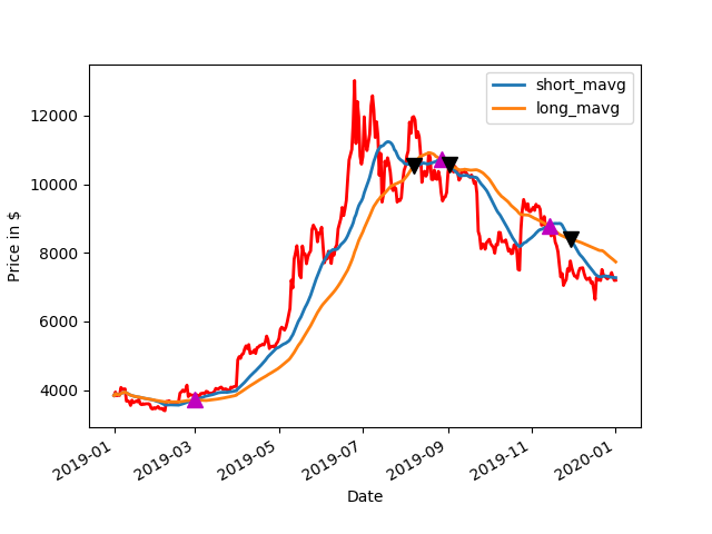
BTC Price with Average and Buy and Sell points
2019 BTC Price with Average and Buy and Sell points Up Arrow = BUY, Down Arrow = SELL
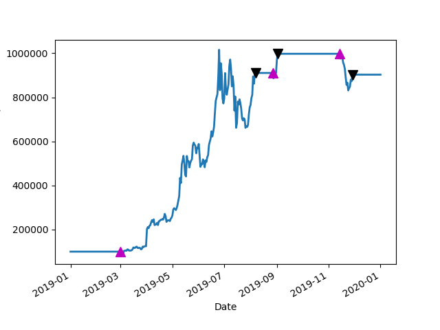
Amount of cash made on paper
2019: Amount of cash made on paper

output from simple-strat-loop-backtest-2019.py

Get Data
Run Model
Short AVG,Long AVG,Best Bank 1 1 100000.0
Short AVG,Long AVG,Best Bank 1 2 611522.802734375
Short AVG,Long AVG,Best Bank 1 4 646585.4736328125
Short AVG,Long AVG,Best Bank 1 16 652523.6328125
Short AVG,Long AVG,Best Bank 1 17 689456.2744140625
Short AVG,Long AVG,Best Bank 3 89 690951.904296875
Short AVG,Long AVG,Best Bank 4 90 696133.9599609375
Short AVG,Long AVG,Best Bank 6 86 707596.8994140625
Short AVG,Long AVG,Best Bank 9 82 709683.1787109375
Short AVG,Long AVG,Best Bank 9 83 732913.4521484375
Short AVG,Long AVG,Best Bank 10 83 742904.150390625
Short AVG,Long AVG,Best Bank 13 17 746094.677734375
Short AVG,Long AVG,Best Bank 14 81 762164.5263671875
Short AVG,Long AVG,Best Bank 22 95 781311.2548828125
Short AVG,Long AVG,Best Bank 27 55 814494.62890625
Short AVG,Long AVG,Best Bank 29 56 820056.7626953125
Short AVG,Long AVG,Best Bank 29 57 886127.4658203125
Short AVG,Long AVG,Best Bank 29 59 902908.9599609375
signal   short_mavg    long_mavg  positions
Date
2019-01-01     0.0  3843.520020  3843.520020        NaN
2019-01-02     0.0  3893.464722  3893.464722        0.0
2019-01-03     0.0  3874.556885  3874.556885        0.0
2019-01-04     0.0  3870.347046  3870.347046        0.0
2019-01-05     0.0  3865.316553  3865.316553        0.0
2019-01-06     0.0  3900.535889  3900.535889        0.0
2019-01-07     0.0  3918.351946  3918.351946        0.0
2019-01-08     0.0  3932.413940  3932.413940        0.0
2019-01-09     0.0  3943.845323  3943.845323        0.0
2019-01-10     0.0  3917.353247  3917.353247        0.0
2019-01-11     0.0  3896.445268  3896.445268        0.0
2019-01-12     0.0  3876.849915  3876.849915        0.0
2019-01-13     0.0  3851.934777  3851.934777        0.0
2019-01-14     0.0  3841.514596  3841.514596        0.0
2019-01-15     0.0  3827.458643  3827.458643        0.0
2019-01-16     0.0  3816.680405  3816.680405        0.0
2019-01-17     0.0  3808.555908  3808.555908        0.0
2019-01-18     0.0  3800.182766  3800.182766        0.0
2019-01-19     0.0  3796.413587  3796.413587        0.0
2019-01-20     0.0  3786.643591  3786.643591        0.0
2019-01-21     0.0  3776.614490  3776.614490        0.0
2019-01-22     0.0  3768.794611  3768.794611        0.0
2019-01-23     0.0  3760.808891  3760.808891        0.0
2019-01-24     0.0  3754.144582  3754.144582        0.0
2019-01-25     0.0  3747.969434  3747.969434        0.0
2019-01-26     0.0  3742.372934  3742.372934        0.0
2019-01-27     0.0  3736.506004  3736.506004        0.0
2019-01-28     0.0  3727.004020  3727.004020        0.0
2019-01-29     0.0  3717.387224  3717.387224        0.0
2019-01-30     0.0  3705.065211  3709.680371        0.0
…            …          …          …        …
2019-12-03     0.0  8139.303778  8350.672074        0.0
2019-12-04     0.0  8067.217824  8338.195445        0.0
2019-12-05     0.0  8001.267056  8324.681624        0.0
2019-12-06     0.0  7941.937231  8313.125919        0.0
2019-12-07     0.0  7898.880573  8295.507233        0.0
2019-12-08     0.0  7855.803442  8278.183023        0.0
2019-12-09     0.0  7798.747340  8262.575270        0.0
2019-12-10     0.0  7747.724289  8244.635676        0.0
2019-12-11     0.0  7692.612742  8225.930954        0.0
2019-12-12     0.0  7638.642797  8206.752102        0.0
2019-12-13     0.0  7589.042447  8190.893042        0.0
2019-12-14     0.0  7541.893538  8175.251465        0.0
2019-12-15     0.0  7493.670814  8159.122492        0.0
2019-12-16     0.0  7436.929603  8141.483051        0.0
2019-12-17     0.0  7379.385776  8118.634824        0.0
2019-12-18     0.0  7347.339473  8102.613207        0.0
2019-12-19     0.0  7318.911065  8084.971233        0.0
2019-12-20     0.0  7304.292666  8070.405356        0.0
2019-12-21     0.0  7300.657530  8064.922082        0.0
2019-12-22     0.0  7304.581391  8065.228863        0.0
2019-12-23     0.0  7315.192130  8043.109003        0.0
2019-12-24     0.0  7321.274835  8010.525266        0.0
2019-12-25     0.0  7323.232927  7971.939519        0.0
2019-12-26     0.0  7313.139935  7937.750000        0.0
2019-12-27     0.0  7307.173811  7901.519506        0.0
2019-12-28     0.0  7291.889211  7869.523975        0.0
2019-12-29     0.0  7286.821037  7839.406482        0.0
2019-12-30     0.0  7282.293541  7806.048696        0.0
2019-12-31     0.0  7277.866329  7769.928041        0.0
2020-01-01     0.0  7273.729391  7735.433461        0.0

[366 rows x 4 columns]
BTC-USD  holdings      cash     total  returns
Date
2019-01-01      0.0       0.0  100000.0  100000.0      NaN
2019-01-02      0.0       0.0  100000.0  100000.0      0.0
2019-01-03      0.0       0.0  100000.0  100000.0      0.0
2019-01-04      0.0       0.0  100000.0  100000.0      0.0
2019-01-05      0.0       0.0  100000.0  100000.0      0.0
BTC-USD  holdings           cash          total  returns
Date
2019-12-28      0.0       0.0  902908.959961  902908.959961      0.0
2019-12-29      0.0       0.0  902908.959961  902908.959961      0.0
2019-12-30      0.0       0.0  902908.959961  902908.959961      0.0
2019-12-31      0.0       0.0  902908.959961  902908.959961      0.0
2020-01-01      0.0       0.0  902908.959961  902908.959961      0.0
Portfolio Plot
Sharpe Ratio 2.2316038135122973
Compound Annual Growth Rate (CAGR) 0.8258754145331861
HODL Gains: 1.8258754145331861


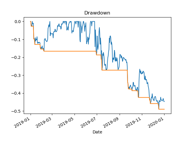
Maximum Drawdown for the Period 1/1/2019-12/31/2019

2018

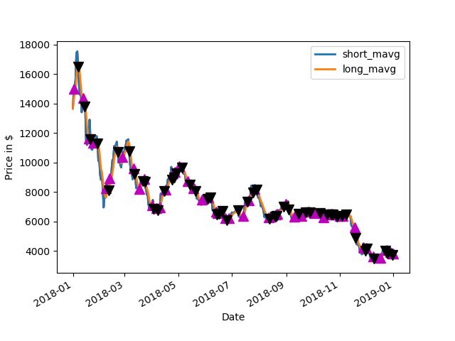
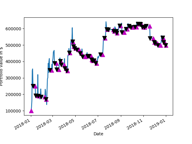
Followup, I was curious about the rough 2018 year for BTC. 2018 was quite bearish, with only a few small rallies up. It had awful buy and hold performance.

HODL Gains: 0.2565408133534354

Short AVG,Long AVG,Best Bank 1 4 498855.46875

Buy and hold would have been a 4x loss and DMAC would have traded in and out quite often, racking up some fees and slippage of course but, made a 5X gain.

2018 BTC Price with Average and Buy and Sell points Up Arrow = BUY, Down Arrow = SELL
 2019: Amount of cash made on paper
2018: Amount of cash made on paper
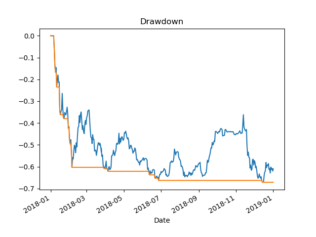
2018 Drawdown
2018 Drawdown

2018 Results Details on Github

Github repo

https://github.com/erickclasen/DMAC-BTC-Trading-Example-With-Tuning

Most Starred Python Projects on Github

I have been working through the Python Crash Course book by Eric Matthes. I got to Chapter 17, Working With API’s  and ran the example code python_repos_updated.py that generates an SVG graph of the most starred Github Python projects. The thing that stands out to me is the amount of machine learning related resources that show up on this hot list. The interactive graph is generated by using Pygal which works well and is easy to use.

Interactive SVG Graph of Most Starred Github Python Projects

Out of curiosity I looked at the most starred C projects on Github as well with a simple modification of the code.

Interactive SVG Graph of the Most Starred Github C Projects

Python Crash Course

The book has been a good resource to develop programming skills in Python, my background is in C primarily and this book was an excellent starting point to officially learn Python. What I mean by that, is that I have been using Python by modding other peoples code when I need some piece of code to use for some application. For a few years I was learning it that way on an as needed basis (plus using the Internet to look up things that I might get suck on) which works to a point. When I started to get into machine learning a bit deeper, I could see that having a more formal introduction to Python would be helpful. Having a book that goes through the process formally helped to quickly build skills in my opinion. In a matter of a few months I have gone through a decent amount of the book and have been able to branch off some of the examples and create free standing code that was interesting to learn from.